Mie Scattering Databases

import sasktran2 as sk
import numpy as np

SASKTRAN2 includes the ability to generate scattering properties for Mie scatterers. Generally a Mie scattering atmospheric constituent is described by a particle size distribution, and a refractive index. Since Mie scattering calculations can be slow, SASKTRAN2 does not contain perform Mie calculations alongside the radiative transfer calculation, instead databases are generated using internal tools that can then be re-used.

Let’s start by creating a Mie scattering database for sulfate aerosols following a log-normal particle distribution parameterized by a median radius and mode width.

mie_db = sk.database.MieDatabase(
    sk.mie.distribution.LogNormalDistribution(),
    sk.mie.refractive.H2SO4(),
    wavelengths_nm=np.arange(270, 1000, 50.0),
    median_radius=[100, 150, 200],
    mode_width=[1.5, 1.7],
)

The main class which provides the database functionality is the sasktran2.database.MieDatabase object. When it is created for the first time the local database will be generated. Any subsequent instantiations of the object will re-use the cached database. In creating the database we provided a sasktran2.mie.distribution.LogNormalDistribution object which defines the particle size distribution for the scatterer, as well as a sasktran2.mie.refractive.H2SO4 which in this case is the refractive index function for sulfates. We also specified the wavelengths to create the database at, as well as the particle size parameters that should be used.

We can look at the created database

mie_db.load_ds()

<xarray.Dataset> Size: 278kB
Dimensions:        (median_radius: 3, mode_width: 2, wavelength_nm: 15,
                    legendre: 64)
Coordinates:
  * median_radius  (median_radius) int64 24B 100 150 200
  * mode_width     (mode_width) float64 16B 1.5 1.7
  * wavelength_nm  (wavelength_nm) float64 120B 270.0 320.0 ... 920.0 970.0
Dimensions without coordinates: legendre
Data variables:
    xs_scattering  (wavelength_nm, median_radius, mode_width) float64 720B ...
    xs_total       (wavelength_nm, median_radius, mode_width) float64 720B ...
    lm_a1          (wavelength_nm, legendre, median_radius, mode_width) float64 46kB ...
    lm_a2          (wavelength_nm, legendre, median_radius, mode_width) float64 46kB ...
    lm_a3          (wavelength_nm, legendre, median_radius, mode_width) float64 46kB ...
    lm_a4          (wavelength_nm, legendre, median_radius, mode_width) float64 46kB ...
    lm_b1          (wavelength_nm, legendre, median_radius, mode_width) float64 46kB ...
    lm_b2          (wavelength_nm, legendre, median_radius, mode_width) float64 46kB ...

xarray.Dataset

• Dimensions:
  • median_radius: 3
  • mode_width: 2
  • wavelength_nm: 15
  • legendre: 64
• Coordinates: (3)
  • median_radius
    (median_radius)
    int64
    100 150 200

    array([100, 150, 200])

  • mode_width
    (mode_width)
    float64
    1.5 1.7

    array([1.5, 1.7])

  • wavelength_nm
    (wavelength_nm)
    float64
    270.0 320.0 370.0 ... 920.0 970.0

    array([270., 320., 370., 420., 470., 520., 570., 620., 670., 720., 770., 820.,
           870., 920., 970.])

• Data variables: (8)
  • xs_scattering
    (wavelength_nm, median_radius, mode_width)
    float64
    ...

    [90 values with dtype=float64]

  • xs_total
    (wavelength_nm, median_radius, mode_width)
    float64
    ...

    [90 values with dtype=float64]

  • lm_a1
    (wavelength_nm, legendre, median_radius, mode_width)
    float64
    ...

    [5760 values with dtype=float64]

  • lm_a2
    (wavelength_nm, legendre, median_radius, mode_width)
    float64
    ...

    [5760 values with dtype=float64]

  • lm_a3
    (wavelength_nm, legendre, median_radius, mode_width)
    float64
    ...

    [5760 values with dtype=float64]

  • lm_a4
    (wavelength_nm, legendre, median_radius, mode_width)
    float64
    ...

    [5760 values with dtype=float64]

  • lm_b1
    (wavelength_nm, legendre, median_radius, mode_width)
    float64
    ...

    [5760 values with dtype=float64]

  • lm_b2
    (wavelength_nm, legendre, median_radius, mode_width)
    float64
    ...

    [5760 values with dtype=float64]

• Indexes: (3)
  • median_radius
    PandasIndex

    PandasIndex(Index([100, 150, 200], dtype='int64', name='median_radius'))

  • mode_width
    PandasIndex

    PandasIndex(Index([1.5, 1.7], dtype='float64', name='mode_width'))

  • wavelength_nm
    PandasIndex

    PandasIndex(Index([270.0, 320.0, 370.0, 420.0, 470.0, 520.0, 570.0, 620.0, 670.0, 720.0,
           770.0, 820.0, 870.0, 920.0, 970.0],
          dtype='float64', name='wavelength_nm'))

• Attributes: (0)

Which contains the scattering and absorption cross sections, as well as the Legendre expansion moments of the phase function that are necessary for the radiative transfer calculation.

Including Mie Scatterers in the Radiative Transfer Calculation

The Mie database can be included and used as an optical property with the standard sasktran2.constituent.NumberDensityScatterer and sasktran2.constituent.ExtinctionScatterer constituents.

First we set up the example calculation without aerosol

import matplotlib.pyplot as plt

config = sk.Config()

altitudes_m = np.arange(0, 65001, 1000)

model_geometry = sk.Geometry1D(cos_sza=0.6,
                               solar_azimuth=0,
                               earth_radius_m=6372000,
                               altitude_grid_m=altitudes_m,
                               interpolation_method=sk.InterpolationMethod.LinearInterpolation,
                               geometry_type=sk.GeometryType.Spherical)

viewing_geo = sk.ViewingGeometry()

for alt in [10000, 20000, 30000, 40000]:
    ray = sk.TangentAltitudeSolar(tangent_altitude_m=alt,
                                    relative_azimuth=45*np.pi/180,
                                    observer_altitude_m=200000,
                                    cos_sza=0.6)
    viewing_geo.add_ray(ray)

wavel = np.arange(280.0, 800.0, 1)

atmosphere = sk.Atmosphere(model_geometry, config, wavelengths_nm=wavel)

sk.climatology.us76.add_us76_standard_atmosphere(atmosphere)

atmosphere['rayleigh'] = sk.constituent.Rayleigh()
atmosphere['ozone'] = sk.climatology.mipas.constituent("O3", sk.optical.O3DBM())

engine = sk.Engine(config, model_geometry, viewing_geo)

radiance_no_aerosol = engine.calculate_radiance(atmosphere)

Now we can add in aerosol, let’s set the extinction to be a constant 1e-7 per metre until 30 km, and then zero above that.

aero_ext = np.zeros(len(altitudes_m))
aero_ext[0:30] = 1e-7

atmosphere['aerosol'] = sk.constituent.ExtinctionScatterer(
    mie_db,
    altitudes_m=altitudes_m,
    extinction_per_m=aero_ext,
    extinction_wavelength_nm=745,
    median_radius=np.ones_like(aero_ext)*120,
    mode_width=np.ones_like(aero_ext)*1.6
)

radiance_with_aerosol = engine.calculate_radiance(atmosphere)

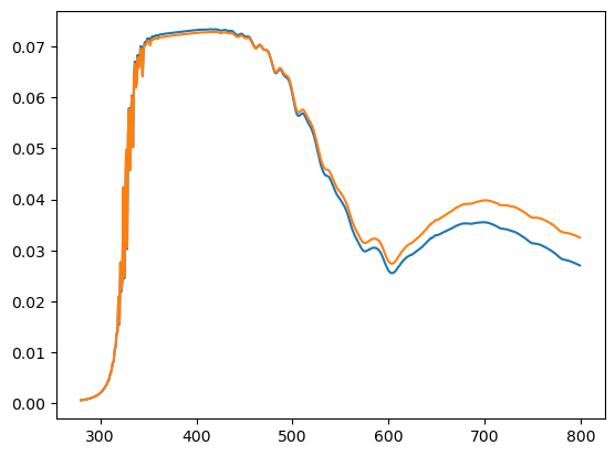
And we can plot the results

plt.plot(
    wavel, radiance_no_aerosol['radiance'].isel(los=0, stokes=0),
    wavel, radiance_with_aerosol['radiance'].isel(los=0, stokes=0)
)

[<matplotlib.lines.Line2D at 0x7f9808b2cc10>,
 <matplotlib.lines.Line2D at 0x7f9808b5ced0>]

If we look at the dataset with aerosol included,

radiance_with_aerosol

<xarray.Dataset> Size: 6MB
Dimensions:                   (wavelength: 520, stokes: 1, altitude: 66,
                               los: 4, ozone_altitude: 50, aerosol_altitude: 66)
Coordinates:
  * wavelength                (wavelength) float64 4kB 280.0 281.0 ... 799.0
  * stokes                    (stokes) <U1 4B 'I'
  * altitude                  (altitude) float64 528B 0.0 1e+03 ... 6.5e+04
Dimensions without coordinates: los, ozone_altitude, aerosol_altitude
Data variables:
    radiance                  (wavelength, los, stokes) float64 17kB 0.000588...
    wf_pressure_pa            (altitude, wavelength, los, stokes) float64 1MB ...
    wf_temperature_k          (altitude, wavelength, los, stokes) float64 1MB ...
    wf_ozone_vmr              (ozone_altitude, wavelength, los, stokes) float64 832kB ...
    wf_aerosol_median_radius  (aerosol_altitude, wavelength, los, stokes) float64 1MB ...
    wf_aerosol_mode_width     (aerosol_altitude, wavelength, los, stokes) float64 1MB ...
    wf_aerosol_extinction     (aerosol_altitude, wavelength, los, stokes) float64 1MB ...

xarray.Dataset

• Dimensions:
  • wavelength: 520
  • stokes: 1
  • altitude: 66
  • los: 4
  • ozone_altitude: 50
  • aerosol_altitude: 66
• Coordinates: (3)
  • wavelength
    (wavelength)
    float64
    280.0 281.0 282.0 ... 798.0 799.0

    array([280., 281., 282., ..., 797., 798., 799.])

  • stokes
    (stokes)
    <U1
    'I'

    array(['I'], dtype='<U1')

  • altitude
    (altitude)
    float64
    0.0 1e+03 2e+03 ... 6.4e+04 6.5e+04

    array([    0.,  1000.,  2000.,  3000.,  4000.,  5000.,  6000.,  7000.,  8000.,
            9000., 10000., 11000., 12000., 13000., 14000., 15000., 16000., 17000.,
           18000., 19000., 20000., 21000., 22000., 23000., 24000., 25000., 26000.,
           27000., 28000., 29000., 30000., 31000., 32000., 33000., 34000., 35000.,
           36000., 37000., 38000., 39000., 40000., 41000., 42000., 43000., 44000.,
           45000., 46000., 47000., 48000., 49000., 50000., 51000., 52000., 53000.,
           54000., 55000., 56000., 57000., 58000., 59000., 60000., 61000., 62000.,
           63000., 64000., 65000.])

• Data variables: (7)
  • radiance
    (wavelength, los, stokes)
    float64
    0.0005884 0.0006233 ... 0.0003526

    array([[[0.00058836],
            [0.00062333],
            [0.00066996],
            [0.00073898]],
    
           [[0.00061794],
            [0.0006551 ],
            [0.00070483],
            [0.00077895]],
    
           [[0.00065769],
            [0.00069775],
            [0.00075162],
            [0.00083258]],
    
           ...,
    
           [[0.03269713],
            [0.01212761],
            [0.00153332],
            [0.00035611]],
    
           [[0.03260514],
            [0.01209395],
            [0.00152593],
            [0.00035433]],
    
           [[0.03251367],
            [0.01206053],
            [0.0015186 ],
            [0.00035255]]])

  • wf_pressure_pa
    (altitude, wavelength, los, stokes)
    float64
    0.0 0.0 0.0 ... 2.255e-08 2.743e-08

    array([[[[0.00000000e+00],
             [0.00000000e+00],
             [0.00000000e+00],
             [0.00000000e+00]],
    
            [[0.00000000e+00],
             [0.00000000e+00],
             [0.00000000e+00],
             [0.00000000e+00]],
    
            [[0.00000000e+00],
             [0.00000000e+00],
             [0.00000000e+00],
             [0.00000000e+00]],
    
            ...,
    
            [[0.00000000e+00],
             [0.00000000e+00],
             [0.00000000e+00],
    ...
             [4.75925367e-07],
             [5.25097006e-07],
             [5.94304846e-07]],
    
            ...,
    
            [[9.30583577e-09],
             [1.66039845e-08],
             [2.27599351e-08],
             [2.77020560e-08]],
    
            [[9.29725028e-09],
             [1.65422198e-08],
             [2.26531387e-08],
             [2.75654990e-08]],
    
            [[9.28878950e-09],
             [1.64809860e-08],
             [2.25471096e-08],
             [2.74298735e-08]]]])

  • wf_temperature_k
    (altitude, wavelength, los, stokes)
    float64
    0.0 0.0 ... -1.033e-09 -1.256e-09

    array([[[[ 0.00000000e+00],
             [ 0.00000000e+00],
             [ 0.00000000e+00],
             [ 0.00000000e+00]],
    
            [[ 0.00000000e+00],
             [ 0.00000000e+00],
             [ 0.00000000e+00],
             [ 0.00000000e+00]],
    
            [[ 0.00000000e+00],
             [ 0.00000000e+00],
             [ 0.00000000e+00],
             [ 0.00000000e+00]],
    
            ...,
    
            [[ 0.00000000e+00],
             [ 0.00000000e+00],
             [ 0.00000000e+00],
    ...
             [-2.30062049e-08],
             [-2.54653394e-08],
             [-2.89801588e-08]],
    
            ...,
    
            [[-4.26244202e-10],
             [-7.60528373e-10],
             [-1.04249533e-09],
             [-1.26886408e-09]],
    
            [[-4.25850953e-10],
             [-7.57699303e-10],
             [-1.03760364e-09],
             [-1.26260923e-09]],
    
            [[-4.25463416e-10],
             [-7.54894552e-10],
             [-1.03274708e-09],
             [-1.25639704e-09]]]])

  • wf_ozone_vmr
    (ozone_altitude, wavelength, los, stokes)
    float64
    0.0 0.0 0.0 0.0 ... 0.0 0.0 0.0 0.0

    array([[[[0.],
             [0.],
             [0.],
             [0.]],
    
            [[0.],
             [0.],
             [0.],
             [0.]],
    
            [[0.],
             [0.],
             [0.],
             [0.]],
    
            ...,
    
            [[0.],
             [0.],
             [0.],
    ...
             [0.],
             [0.],
             [0.]],
    
            ...,
    
            [[0.],
             [0.],
             [0.],
             [0.]],
    
            [[0.],
             [0.],
             [0.],
             [0.]],
    
            [[0.],
             [0.],
             [0.],
             [0.]]]])

  • wf_aerosol_median_radius
    (aerosol_altitude, wavelength, los, stokes)
    float64
    0.0 0.0 0.0 0.0 ... 0.0 0.0 0.0 0.0

    array([[[[0.],
             [0.],
             [0.],
             [0.]],
    
            [[0.],
             [0.],
             [0.],
             [0.]],
    
            [[0.],
             [0.],
             [0.],
             [0.]],
    
            ...,
    
            [[0.],
             [0.],
             [0.],
    ...
             [0.],
             [0.],
             [0.]],
    
            ...,
    
            [[0.],
             [0.],
             [0.],
             [0.]],
    
            [[0.],
             [0.],
             [0.],
             [0.]],
    
            [[0.],
             [0.],
             [0.],
             [0.]]]])

  • wf_aerosol_mode_width
    (aerosol_altitude, wavelength, los, stokes)
    float64
    0.0 0.0 0.0 0.0 ... 0.0 0.0 0.0 0.0

    array([[[[0.],
             [0.],
             [0.],
             [0.]],
    
            [[0.],
             [0.],
             [0.],
             [0.]],
    
            [[0.],
             [0.],
             [0.],
             [0.]],
    
            ...,
    
            [[0.],
             [0.],
             [0.],
    ...
             [0.],
             [0.],
             [0.]],
    
            ...,
    
            [[0.],
             [0.],
             [0.],
             [0.]],
    
            [[0.],
             [0.],
             [0.],
             [0.]],
    
            [[0.],
             [0.],
             [0.],
             [0.]]]])

  • wf_aerosol_extinction
    (aerosol_altitude, wavelength, los, stokes)
    float64
    0.0 0.0 0.0 ... 839.5 1.018e+03

    array([[[[   0.        ],
             [   0.        ],
             [   0.        ],
             [   0.        ]],
    
            [[   0.        ],
             [   0.        ],
             [   0.        ],
             [   0.        ]],
    
            [[   0.        ],
             [   0.        ],
             [   0.        ],
             [   0.        ]],
    
            ...,
    
            [[   0.        ],
             [   0.        ],
             [   0.        ],
    ...
             [ 756.28073937],
             [ 857.24920782],
             [1014.26455491]],
    
            ...,
    
            [[ 402.182019  ],
             [ 635.69934664],
             [ 841.98940053],
             [1021.65399293]],
    
            [[ 402.55217529],
             [ 635.23740237],
             [ 840.74311051],
             [1019.92337112]],
    
            [[ 402.91653315],
             [ 634.77457805],
             [ 839.49506185],
             [1018.18918291]]]])

• Indexes: (3)
  • wavelength
    PandasIndex

    PandasIndex(Index([280.0, 281.0, 282.0, 283.0, 284.0, 285.0, 286.0, 287.0, 288.0, 289.0,
           ...
           790.0, 791.0, 792.0, 793.0, 794.0, 795.0, 796.0, 797.0, 798.0, 799.0],
          dtype='float64', name='wavelength', length=520))

  • stokes
    PandasIndex

    PandasIndex(Index(['I'], dtype='object', name='stokes'))

  • altitude
    PandasIndex

    PandasIndex(Index([    0.0,  1000.0,  2000.0,  3000.0,  4000.0,  5000.0,  6000.0,  7000.0,
            8000.0,  9000.0, 10000.0, 11000.0, 12000.0, 13000.0, 14000.0, 15000.0,
           16000.0, 17000.0, 18000.0, 19000.0, 20000.0, 21000.0, 22000.0, 23000.0,
           24000.0, 25000.0, 26000.0, 27000.0, 28000.0, 29000.0, 30000.0, 31000.0,
           32000.0, 33000.0, 34000.0, 35000.0, 36000.0, 37000.0, 38000.0, 39000.0,
           40000.0, 41000.0, 42000.0, 43000.0, 44000.0, 45000.0, 46000.0, 47000.0,
           48000.0, 49000.0, 50000.0, 51000.0, 52000.0, 53000.0, 54000.0, 55000.0,
           56000.0, 57000.0, 58000.0, 59000.0, 60000.0, 61000.0, 62000.0, 63000.0,
           64000.0, 65000.0],
          dtype='float64', name='altitude'))

• Attributes: (0)

We can see that the model has also calculated the derivatives with respect to the particle size parameters, median_radius and mode_width.