Quick Start

import sasktran2 as sk

SASKTRAN2 requires four things in order to perform the radiative transfer calculation

• A configuration object which stores user options, sasktran2.Config

• A specification of the model geometry, and a global grid where atmospheric parameters are specified on. This is handled by the sasktran2.Geometry1D object

• A sasktran2.ViewingGeometry object that specifies the viewing conditions we want output at.

• A sasktran2.Atmosphere class that defines the atmospheric state

The Configuration object

The sasktran2.Config object stores all of the user configuration options that are necessary for the calculation,

config = sk.Config()

The default configuration object contains setting for a single scattering atmosphere. Let’s add a multiple scattering source

config.multiple_scatter_source = sk.MultipleScatterSource.DiscreteOrdinates

To speed up the calculation let’s also adjust some accuracy settings

config.num_streams = 2

The Model Geometry

The model geometry is the grid that the radiative transfer calculation is actually performed on. Usually this involves specifying the coordinates (spherical, plane parallel, etc.) the number of dimensions the atmosphere is allowed to vary in (1, 2, 3), as well as the actual grid values themselves. Sometimes an internal definition of a reference point is also required to provide context to the viewing geometry policies.

Similar to other SASKTRAN2 components, there are multiple ways to construct the model geometry. The standard one, and the one you probably want, is sasktran2.Geometry1D,

import numpy as np

model_geometry = sk.Geometry1D(cos_sza=0.6,
                                solar_azimuth=0,
                                earth_radius_m=6372000,
                                altitude_grid_m=np.arange(0, 65001, 1000),
                                interpolation_method=sk.InterpolationMethod.LinearInterpolation,
                                geometry_type=sk.GeometryType.Spherical)

The Viewing Geometry

We specify radiance output through a list of single positions and look vectors. These are stored inside the sasktran2.ViewingGeometry object.

viewing_geo = sk.ViewingGeometry()

We can add a set of four limb viewing lines of sight through,

for alt in [10000, 20000, 30000, 40000]:
    ray = sk.TangentAltitudeSolar(tangent_altitude_m=alt,
                                    relative_azimuth=0,
                                    observer_altitude_m=200000,
                                    cos_sza=0.6)
    viewing_geo.add_ray(ray)

The Atmospheric State

We start by constructing our sasktran2.Atmosphere object,

wavel = np.arange(280.0, 800.0, 0.1)
atmosphere = sk.Atmosphere(model_geometry, config, wavelengths_nm=wavel)

In SASKTRAN2 calculations are most efficiently performed over a spectral dimension, here we have specified wavelength, but in practice this can be any dimension we want to vectorize the calculation over.

The easiest way to specify the atmosphere is through what we call the constituent interface, essentially the atmosphere is composed of discrete constituents each providing their own input to the atmospheric state.

To add Rayleigh scattering we can do,

atmosphere['rayleigh'] = sk.constituent.Rayleigh()

SASKTRAN2 contains built in climatologies (sasktran2.climatology.*) of some atmospheric constituents to aid in setting up calculations quickly. Here we add absorption due to ozone and nitrogen dioxide,

atmosphere['ozone'] = sk.climatology.mipas.constituent("O3", sk.optical.O3DBM())
atmosphere['no2'] = sk.climatology.mipas.constituent("NO2", sk.optical.NO2Vandaele())

many atmospheric constituents require databases of cross sections and optionally scattering properties, in SASKTRAN2 we refer to these as optical properties, and they are contained in the sasktran2.optical namespace.

Lastly, many constituents require that the pressure and temperature of the atmosphere be known to compute background number density and evaluate cross sections at the appropriate atmospheric conditions. These can be set directly with the sasktran2.Atmosphere.pressure_pa and sasktran2.Atmosphere.temperature_k properties, or they can be set through built in climatologies such as

sk.climatology.us76.add_us76_standard_atmosphere(atmosphere)

Performing the Calculation

The radiative transfer calculation is done through the sasktran2.Engine object,

engine = sk.Engine(config, model_geometry, viewing_geo)

Upon construction, all of the geometry information is calculated and cached. In order to do the actual calculation, we pass in the sasktran2.Atmosphere object

output = engine.calculate_radiance(atmosphere)

The default output format is an xarray.Dataset object containing relevant fields including radiance and derivatives of the radiance with respect to atmospheric parameters.

print(output)

<xarray.Dataset> Size: 50MB
Dimensions:               (wavelength: 5200, los: 4, stokes: 1, altitude: 66,
                           ozone_altitude: 50, no2_altitude: 50)
Coordinates:
  * wavelength            (wavelength) float64 42kB 280.0 280.1 ... 799.8 799.9
  * stokes                (stokes) <U1 4B 'I'
Dimensions without coordinates: los, altitude, ozone_altitude, no2_altitude
Data variables:
    radiance              (wavelength, los, stokes) float64 166kB 0.0007154 ....
    wf_temperature_k      (altitude, wavelength, los, stokes) float64 11MB -1...
    wf_pressure_pa        (altitude, wavelength, los, stokes) float64 11MB 2....
    wf_ozone_vmr          (ozone_altitude, wavelength, los, stokes) float64 8MB ...
    wf_specific_humidity  (altitude, wavelength, los, stokes) float64 11MB 2....
    wf_no2_vmr            (no2_altitude, wavelength, los, stokes) float64 8MB ...

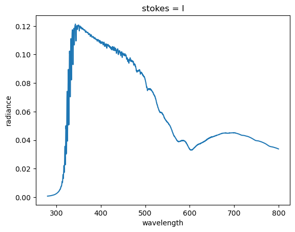
We can plot the output directly,

output['radiance'].isel(los=0).plot()

[<matplotlib.lines.Line2D at 0x7dcfef0aa7b0>]

Note

All calculations in SASKTRAN2 unless explicitly stated assume an incident solar irradiance of 1. Therefore the output units of radiance are [/steradian]