Specifying Aerosols and Clouds

import sasktran2 as sk
import numpy as np
import matplotlib.pyplot as plt

Aerosols and clouds in sasktran2 are specified through a combination of two things:

• The amount of aerosol/cloud, this could be a vertical optical depth, extinction at a given reference wavelength, or a number density

• The optical properties of the scatterer

As an example, we will start with a clear sky radiative transfer calculation and add in a cloud,

import sasktran2 as sk
import numpy as np
import matplotlib.pyplot as plt

config = sk.Config()
config.multiple_scatter_source = sk.MultipleScatterSource.DiscreteOrdinates
config.num_streams = 2
config.delta_m_scaling = True

altitude_grid = np.arange(0, 65001, 1000)

model_geometry = sk.Geometry1D(cos_sza=0.6,
                               solar_azimuth=0,
                               earth_radius_m=6372000,
                               altitude_grid_m=altitude_grid,
                               interpolation_method=sk.InterpolationMethod.LinearInterpolation,
                               geometry_type=sk.GeometryType.PlaneParallel)

viewing_geo = sk.ViewingGeometry()

viewing_geo.add_ray(
    sk.GroundViewingSolar(
        cos_sza=0.6,
        relative_azimuth=0,
        cos_viewing_zenith=0.8,
        observer_altitude_m=200000,
    )
)

wavel = np.arange(300, 800, 0.1)
atmosphere = sk.Atmosphere(model_geometry, config, wavelengths_nm=wavel)

atmosphere.surface.albedo[:] = 0.3

sk.climatology.us76.add_us76_standard_atmosphere(atmosphere)

atmosphere["rayleigh"] = sk.constituent.Rayleigh()
atmosphere['ozone'] = sk.climatology.mipas.constituent("O3", sk.optical.O3DBM())
atmosphere['no2'] = sk.climatology.mipas.constituent("NO2", sk.optical.NO2Vandaele())

engine = sk.Engine(config, model_geometry, viewing_geo)

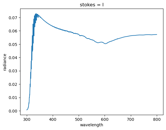
radiance_no_cloud = engine.calculate_radiance(atmosphere)

radiance_no_cloud["radiance"].isel(los=0).plot()

[<matplotlib.lines.Line2D at 0x70d9e9d8c5f0>]

Next, we will create an optical property by specifying the single scattering albedo and asymmetry factors,

wavel = np.arange(300, 801, 10.0)
xsec = np.ones_like(wavel)
ssa = np.ones_like(wavel) * 1.0
g = np.ones_like(wavel) * 0.75

hg = sk.optical.HenyeyGreenstein.from_parameters(
    wavelength_nm=wavel,
    xs_total=xsec,
    ssa=ssa,
    g=g,
)

And we will specify the cloud with a Gaussian height profile and add it to the atmosphere,

cloud = sk.constituent.GaussianHeightExtinction(
    optical_property=hg,
    height_m=2000,
    width_fwhm_m=500,
    vertical_optical_depth=10,
    vertical_optical_depth_wavel_nm=550,
    altitudes_m=altitude_grid,
)

atmosphere["cloud"] = cloud

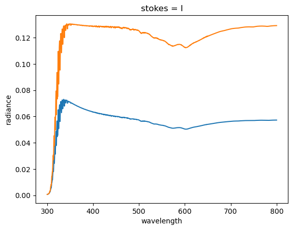
Then we can rerun the calculation

radiance_cloud = engine.calculate_radiance(atmosphere)

radiance_no_cloud["radiance"].isel(los=0).plot()
radiance_cloud["radiance"].isel(los=0).plot()

[<matplotlib.lines.Line2D at 0x70d9e9c0bce0>]

Scatterer optical properties

The following are the supported ways to specify the optical properties of scatterers.

sasktran2.optical.henyey.HenyeyGreenstein([...])	An optical property that uses a Henyey-Greenstein phase function.
sasktran2.optical.database.OpticalDatabaseGenericScattererRust(...)	A purely scattering optical property defined by a database file.
sasktran2.optical.mie.Mie(...)	Mie scattering optical property where the Mie calculations are done on the fly.
sasktran2.database.MieDatabase(...[, ...])	A MieDatabase is a database that caches Mie scattering data on the local file system.

Scattering Constituents

The following are the supported ways to specify the amount of scatterers.

sasktran2.constituent.ExtinctionScatterer(...)	A scattering constituent that is defined by a number density on an altitude grid and an optical property
sasktran2.constituent.NumberDensityScatterer(...)	A scattering constituent that is defined by a number density on an altitude grid and an optical property
sasktran2.constituent.GaussianHeightExtinction(...)	A constituent that is defined by a gaussian-shaped extinction profile.