

Polarized Calculations#
import sasktran2 as sk
SASKTRAN2 supports polarization through changing the sasktran2.Config.num_stokes parameter which
controls the number of Stokes parameters used in the calculation.
config = sk.Config()

print(config.num_stokes)
1
By default this parameter is set to 1.
Setting,
config.num_stokes = 3
is the recommended way to enable the polarization calculation. num_stokes=3 is an approximation
where the V (circular polarization) component is assumed to be 0, which is generally a very good
approximation for Earth’s atmosphere.
Running a Calculation#
Generally the only thing that has to be changed to run a polarized calculation is to set the
sasktran2.Config.num_stokes setting. Here we repeat the same example done in the quickstart
guide but with polarization enabled
import numpy as np
import matplotlib.pyplot as plt

config = sk.Config()
config.num_stokes = 3
config.multiple_scatter_source = sk.MultipleScatterSource.DiscreteOrdinates
config.num_streams = 4

model_geometry = sk.Geometry1D(cos_sza=0.6,
                                solar_azimuth=0,
                                earth_radius_m=6372000,
                                altitude_grid_m=np.arange(0, 65001, 1000),
                                interpolation_method=sk.InterpolationMethod.LinearInterpolation,
                                geometry_type=sk.GeometryType.Spherical)

viewing_geo = sk.ViewingGeometry()

for alt in [10000, 20000, 30000, 40000]:
    ray = sk.TangentAltitudeSolar(tangent_altitude_m=alt,
                                    relative_azimuth=45*np.pi/180,
                                    observer_altitude_m=200000,
                                    cos_sza=0.6)
    viewing_geo.add_ray(ray)

wavel = np.arange(280.0, 800.0, 1)

atmosphere = sk.Atmosphere(model_geometry, config, wavelengths_nm=wavel)

sk.climatology.us76.add_us76_standard_atmosphere(atmosphere)

atmosphere['rayleigh'] = sk.constituent.Rayleigh()

atmosphere['ozone'] = sk.climatology.mipas.constituent("O3", sk.optical.O3DBM())

atmosphere['no2'] = sk.climatology.mipas.constituent("NO2", sk.optical.NO2Vandaele())

engine = sk.Engine(config, model_geometry, viewing_geo)

radiance = engine.calculate_radiance(atmosphere)
Then if we look at the output,
print(radiance)
<xarray.Dataset> Size: 15MB
Dimensions:               (wavelength: 520, los: 4, stokes: 3, altitude: 66,
                           no2_altitude: 50, ozone_altitude: 50)
Coordinates:
  * wavelength            (wavelength) float64 4kB 280.0 281.0 ... 798.0 799.0
  * stokes                (stokes) <U1 12B 'I' 'Q' 'U'
Dimensions without coordinates: los, altitude, no2_altitude, ozone_altitude
Data variables:
    radiance              (wavelength, los, stokes) float64 50kB 0.0005855 .....
    wf_temperature_k      (altitude, wavelength, los, stokes) float64 3MB -9....
    wf_no2_vmr            (no2_altitude, wavelength, los, stokes) float64 2MB ...
    wf_pressure_pa        (altitude, wavelength, los, stokes) float64 3MB 2.6...
    wf_ozone_vmr          (ozone_altitude, wavelength, los, stokes) float64 2MB ...
    wf_specific_humidity  (altitude, wavelength, los, stokes) float64 3MB 1.5...
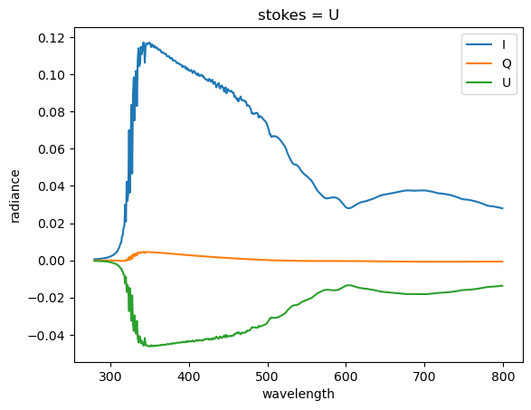
we see that the radiance, as well as the weighting functions, contain 3 Stokes vector elements. We can look at them,
radiance["radiance"].sel(stokes="I").isel(los=0).plot()
radiance["radiance"].sel(stokes="Q").isel(los=0).plot()
radiance["radiance"].sel(stokes="U").isel(los=0).plot()

plt.legend(["I", "Q", "U"])
<matplotlib.legend.Legend at 0x77093015a330>
Stokes Conventions and Basis#
If you only care about the intensity, \(I\), or the degree of linear polarization, \(\frac{\sqrt{Q^2 + U^2}}{I}\), then you can stop reading this section as these quantities do not depend on the Stokes basis.
However, if you need the Stokes parameters \(Q\), \(U\) directly to calculate things like the linearly polarized component \(\frac{I \pm Q}{2}\) then unfortunately you have to read on as the Stokes parameters \(Q\) and \(U\) are only unique when a reference basis has been specified.
Stokes Basis#
By default SASKTRAN2 returns back Stokes vectors in what can only be described as the “standard” basis. This is the basis that every textbook on polarized radiative transfer uses, and extreme amounts of detail can be found in Section 4.3 of
Mishchenko, Michael I., Larry D. Travis, and Andrew A. Lacis. Scattering, absorption, and emission of light by small particles. Cambridge university press, 2002.
or Section 3.2 of
Hovenier, Joop W., Cornelis VM Van der Mee, and Helmut Domke. Transfer of polarized light in planetary atmospheres: basic concepts and practical methods. Vol. 318. Springer Science & Business Media, 2004.
Briefly what this means is that the Stokes reference is implicitly formed from the \(z\)-axis and the look vector. Therefore, if you oriented a horizontal polarizer with the plane formed by the \(z\)-axis and the look vector you would measure, \(\frac{I+Q}{2}\), and likewise a vertical polarizer would measure \(\frac{I-Q}{2}\). This is the default basis mode, but it can be explicitly set with
config.stokes_basis = sk.StokesBasis.Standard
SASKTRAN2 also supports two other Stokes basis conventions. The first is the “observer” basis, set with
config.stokes_basis = sk.StokesBasis.Observer
Here the Stokes reference is in the plane formed by the observer position and the look vector. I.e. if you orient a polarizer in this plane you will measure \(\frac{I \pm Q}{2}\). Often this is a convenient basis when working with instruments since the polarization orientation is often known relative to the observer position vector. However sometimes care must be taken since the observer position in the model may not be exactly what you expect due to conversions between “true” coordinates and the coordinate system used internally in the model.
The last supported basis is the “solar” basis,
config.stokes_basis = sk.StokesBasis.Solar
where the reference plane is defined by the plane spanned by the look vector and the solar vector. This has the advantage that in single scatter, all of the polarization information is stored inside \(Q\), and \(U\) is identically 0. The solar basis can be useful for theoretical calculations.
Basis Summary#
sasktran2.StokesBasis.StandardPolarization reference oriented in the global
z-axis and look vector planesasktran2.StokesBasis.ObserverPolarization reference oriented in the observer position and look vector plane
sasktran2.StokesBasis.SolarPolarization reference oriented in the solar vector and look vector plane
Stokes Conventions#
It is somewhat well-known that even if radiative transfer models state that they use the same Stokes vector basis, they often differ in the sign of \(Q, U, \) or \(V\). The sign of \(V\) is ambiguous, and often different between authors because it can change depending on how the time dependence of the electric field is handled. However every textbook the SASKTRAN2 authors have analyzed uses the same Stokes vector conventions for \(Q\) and \(U\). Typically the sign differences are a result of misunderstandings, for example, the Stokes vector rotation matrix is usually written in terms of angle ``measured clockwise when looking in the direction of propagation’’. It is very easy to make a sign mistake since angles are usually measured counter-clockwise, and also the direction of propagation may be negative of what is internally used inside the model. To further emphasize how easy it is to make a sign-error, in SASKTRAN version 1 \(Q\) was negative that of most other models, and this was eventually traced back to two separate misinterpretations of the Stokes vector equations.
We are very confident that SASKTRAN2 has the correct sign for the \(Q\) and \(U\) components, and agrees with other models that have extensively checked this such as SCIATRAN. The sign of \(Q\) and \(U\) also agree with classic benchmark sources such as the Coulsen tables.
Supported Number of Stokes Parameters#
Currently SASKTRAN2 supports
num_stokes=1Scalar mode, only the \(I\) component of the Stokes vector is calculated. Default.
num_stokes=3Vector mode, the [\(I\), \(Q\), \(U\)] components of the Stokes vector is calculated. Default.