Emissions

To include any type of emissions as part of the radiation source, they must first be enabled in the configuration.

SASKTRAN supports emissions in two ways. The first is the sk.EmissionSource.Standard and is recommended when atmospheric scattering can be neglected, or when working in spherical geometry.

import sasktran2 as sk

config = sk.Config()
config.emission_source = sk.EmissionSource.Standard

When atmospheric scattering is important (e.g. clouds or large amounts of aerosols are present) the Discrete Ordinates source term can be used to handle coupling between emission and scttering

import sasktran2 as sk

config = sk.Config()
config.single_scatter_source = sk.SingleScatterSource.DiscreteOrdinates
config.multiple_scatter_source = sk.MultipleScatterSource.DiscreteOrdinates
config.emission_source = sk.EmissionSource.DiscreteOrdinates

Note that this source only works in plane parallel (or pseudo-spherical) geometry.

As a general rule of thumb, use sk.EmissionSource.Standard in spherical geometry, and sk.EmissionSource.DiscreteOrdinates in plane parallel geometry.

By default, sasktran2.Config.emission_source is set to sk.EmissionSource.NoSource, where emissions are not added to the source and any emissions present in the model atmosphere will be ignored.

Thermal Emissions

After enabling emissions in the configuration, we must also specify the type of emissions to include in the atmosphere. Currently, thermal emissions from the surface and atmosphere are supported. First we will enable emission sources in the configuration and disable the single scatter source.

import matplotlib.pyplot as plt
import numpy as np
import sasktran2 as sk

config = sk.Config()
config.single_scatter_source = sk.SingleScatterSource.NoSource
config.emission_source = sk.EmissionSource.Standard

Now, set up a line of sight that ends at the ground.

model_geometry = sk.Geometry1D(cos_sza=0.6,
                                solar_azimuth=0,
                                earth_radius_m=6372000,
                                altitude_grid_m=np.arange(0, 100001, 1000),
                                interpolation_method=sk.InterpolationMethod.LinearInterpolation,
                                geometry_type=sk.GeometryType.Spherical)

viewing_geo = sk.ViewingGeometry()

ray = sk.GroundViewingSolar(0.6, 0, 0.8, 200000)
viewing_geo.add_ray(ray)

Next, we will add an absorbing/emitting species to the atmosphere. For this example we will use methane, with the cross sections calculated using the HITRAN database. Note that the cross section calculation will take several minutes the first time it runs but the result is saved in a database cache in order to speed up future calculations. The hitran-api python package must be installed to download the database files.

wavelengths = np.arange(7370, 7380, 0.01)

hitran_db = sk.database.HITRANDatabase(
    molecule="CH4",
    start_wavenumber=1355,
    end_wavenumber=1357,
    wavenumber_resolution=0.01,
    reduction_factor=1,
    backend="sasktran2",
    profile="voigt"
)

Now we will create the atmopshere object and enable both line of sight and surface emissions. For the ground emission, we need to specify the surface temperature and emissivity. Wavelength-dependent emissivities can be specified by passing an array of values to the sasktran2.constituent.SurfaceThermalEmission constructor. The array must be the same length as the wavelength array given to the sasktran2.Atmosphere object.

atmosphere = sk.Atmosphere(model_geometry, config, wavelengths_nm=wavelengths, calculate_derivatives=False)

sk.climatology.us76.add_us76_standard_atmosphere(atmosphere)
atmosphere['ch4'] = sk.climatology.mipas.constituent('CH4', hitran_db)
atmosphere['emission'] = sk.constituent.ThermalEmission()
atmosphere['surface_emission'] = atmosphere['surface_emission'] = sk.constituent.SurfaceThermalEmission(temperature_k=300, emissivity=0.9)

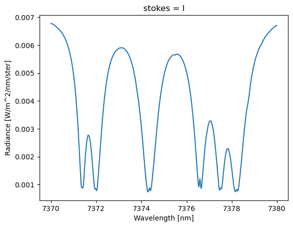
Lastly, perform the calculation and plot the result.

engine = sk.Engine(config, model_geometry, viewing_geo)
rad = engine.calculate_radiance(atmosphere)

rad.isel(stokes=0)["radiance"].plot()
plt.xlabel('Wavelength [nm]')
plt.ylabel('Radiance [W/m^2/nm/ster]')

Text(0, 0.5, 'Radiance [W/m^2/nm/ster]')

Combining Thermal Emissions and Solar Irradiance

If we wish to perform calculations that include both thermal emissions and scattered sunlight, we must take care to ensure that the units of the thermal and solar sources are in agreement. By default, the solar source terms are normalized by the irradiance at the top of the atmosphere, but thermal emissions are input to sasktran with absolute radiance units (W/m^2/nm/ster). To combine these sources we must add the solar irradiance constituent to the atmosphere which changes the units to match the thermal emissions.

atmosphere["solar_irradiance"] = sk.constituent.SolarIrradiance()

See Solar Irradiance documentation for more details.

The Discrete Ordinates Thermal Source

As mentioned above, the Discrete Ordinates thermal source term is capable of including coupling betwene scattering and emission sources. It is only suitable in the Plane Parallel geometry (or pseudo-spherical geometry) currently.

Here we repeat the above example with the Discrete Ordinates source term instead.

import sasktran2 as sk
import matplotlib.pyplot as plt
import numpy as np

config = sk.Config()
config.single_scatter_source = sk.SingleScatterSource.DiscreteOrdinates
config.multiple_scatter_source = sk.MultipleScatterSource.DiscreteOrdinates
config.emission_source = sk.EmissionSource.DiscreteOrdinates

config.num_streams = 4

model_geometry = sk.Geometry1D(cos_sza=0.6,
                                solar_azimuth=0,
                                earth_radius_m=6372000,
                                altitude_grid_m=np.arange(0, 100001, 1000),
                                interpolation_method=sk.InterpolationMethod.LinearInterpolation,
                                geometry_type=sk.GeometryType.PlaneParallel)

viewing_geo = sk.ViewingGeometry()

ray = sk.GroundViewingSolar(0.6, 0, 0.8, 200000)
viewing_geo.add_ray(ray)

wavelengths = np.arange(7370, 7380, 0.01)

hitran_db = sk.database.HITRANDatabase(
    molecule="CH4",
    start_wavenumber=1355,
    end_wavenumber=1357,
    wavenumber_resolution=0.01,
    reduction_factor=1,
    backend="sasktran2",
    profile="voigt"
)

atmosphere = sk.Atmosphere(model_geometry, config, wavelengths_nm=wavelengths, calculate_derivatives=False)

sk.climatology.us76.add_us76_standard_atmosphere(atmosphere)
atmosphere['ch4'] = sk.climatology.mipas.constituent('CH4', hitran_db)
atmosphere['emission'] = sk.constituent.ThermalEmission()
atmosphere['surface_emission'] = atmosphere['surface_emission'] = sk.constituent.SurfaceThermalEmission(temperature_k=300, emissivity=0.9)

engine = sk.Engine(config, model_geometry, viewing_geo)
rad = engine.calculate_radiance(atmosphere)

rad.isel(stokes=0)["radiance"].plot()
plt.xlabel('Wavelength [nm]')
plt.ylabel('Radiance [W/m^2/nm/ster]')

Text(0, 0.5, 'Radiance [W/m^2/nm/ster]')

In this case the results are almost identical because the atmosphere does not contain any scatterers.