Photochemical Emission

SASKTRAN2 has basic support for some photochemical based emission sources. This is enabled by setting

import sasktran2 as sk

config = sk.Config()
config.emission_source = sk.EmissionSource.VolumeEmissionRate

note that it is not currently possible to combine thermal emissions with other photo-chemical based emissions.

Monochromatic Sources

Many photochemical sources in the atmosphere are essentially monochromatic, and can be included by using the sasktran2.constituent.MonochromaticVolumeEmissionRate constituent.

import sasktran2 as sk
import numpy as np
import matplotlib.pyplot as plt

config = sk.Config()
config.emission_source = sk.EmissionSource.VolumeEmissionRate

model_geometry = sk.Geometry1D(cos_sza=-0.6,
                                solar_azimuth=0,
                                earth_radius_m=6372000,
                                altitude_grid_m=np.arange(0, 120001, 1000),
                                interpolation_method=sk.InterpolationMethod.LinearInterpolation,
                                geometry_type=sk.GeometryType.Spherical)

viewing_geo = sk.ViewingGeometry()

for alt in [95000]:
    ray = sk.TangentAltitudeSolar(tangent_altitude_m=alt,
                                    relative_azimuth=0,
                                    observer_altitude_m=200000,
                                    cos_sza=-0.6)
    viewing_geo.add_ray(ray)

wavel = np.arange(556.0, 560.0, 0.01)
atmosphere = sk.Atmosphere(model_geometry, config, wavelengths_nm=wavel)

sk.climatology.us76.add_us76_standard_atmosphere(atmosphere)

# Oxygen green line VER profile
altitude = np.array([
    140, 135, 130, 125, 120, 115, 110,
    105, 100,  95,  90,  85
]).astype(np.float64)[::-1] * 1000

# VER in ph cm^-3 s^-1
VER = np.array([
     400,   600,   800,  1100,  1500,  2000,  2600,
    3200,  3800,  4300,  3600,   900
])[::-1] / 100 # convert to ph cm^-2 m^-1

atmosphere["rayleigh"] = sk.constituent.Rayleigh()
atmosphere["ver"] = sk.constituent.MonochromaticVolumeEmissionRate(altitude, VER, 557.7)

engine = sk.Engine(config, model_geometry, viewing_geo)
output = engine.calculate_radiance(atmosphere)

output["radiance"].isel(los=0).plot()

[<matplotlib.lines.Line2D at 0x75b7e0c2d490>]

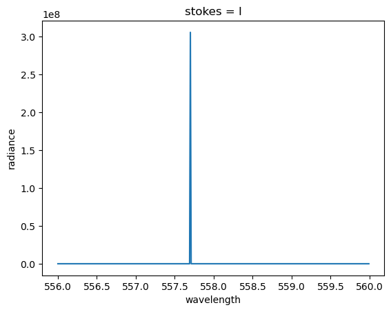
Note that since the calculation must be performed on a finite resolution spectral grid, SASKTRAN internally “widens” the monochromatic line based on the resolution of the calculation. This is done so that integrals over the line produce the correct integrated radiance profile.