Mie Scattering Databases

import sasktran2 as sk
import numpy as np
import matplotlib.pyplot as plt

SASKTRAN2 includes the ability to generate scattering properties for Mie scatterers. Generally a Mie scattering atmospheric constituent is described by a particle size distribution, and a refractive index. Since Mie scattering calculations can be slow, SASKTRAN2 does not contain perform Mie calculations alongside the radiative transfer calculation, instead databases are generated using internal tools that can then be re-used.

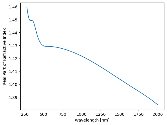
Mie scatterers are parameterized by two quantities, the refractive index, and a particle size distribution. SASKTRAN2 contains several built in refractive index functions (see Refractive Index Containers), let’s create one for sulfates, sasktran2.mie.refractive.H2SO4

refrac = sk.mie.refractive.H2SO4()

wavelengths = np.arange(280, 2000, 0.1)
plt.plot(wavelengths, np.real(refrac.refractive_index(wavelengths)))
plt.xlabel("Wavelength [nm]")
plt.ylabel("Real Part of Refractive Index")

Text(0, 0.5, 'Real Part of Refractive Index')

it is also possible to define your own refractive index entirely using the sasktran2.mie.refractive.RefractiveIndex object.

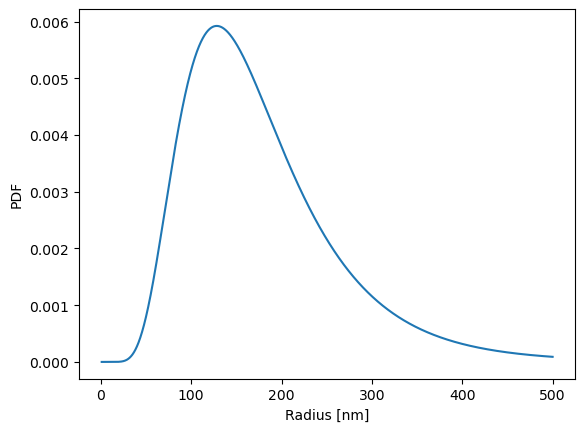
The second quantity that we need is a particle size distribution (see Particle Size Distributions). Here we will create a log-normal particle size distribution

distribution = sk.mie.distribution.LogNormalDistribution()

Every particle size distribution is parameterized by several parameters, we can look at them explicity,

distribution.args()

['median_radius', 'mode_width']

And we can also inspect the distribution for specific values of the parameters (median_radius, mode_width)

radii = np.arange(1, 500, 0.1)
plt.plot(radii, distribution.distribution(median_radius=160, mode_width=1.6).pdf(radii))
plt.xlabel("Radius [nm]")
plt.ylabel("PDF")

Text(0, 0.5, 'PDF')

Now that we have a particle size distribution and a refractive index, we can create our Mie scattering database.

mie_db = sk.database.MieDatabase(
    distribution,
    refrac,
    wavelengths_nm=np.arange(270, 1000, 50.0),
    median_radius=[100, 150, 200],
    mode_width=[1.5, 1.7],
)

The database is a function of wavelength, and any arguments of the particle size distribution, median_radius and mode_width in our case. When it is created for the first time the local database will be generated. Any subsequent instantiations of the object will re-use the cached database.

We can look at the created database

mie_db.load_ds()

<xarray.Dataset> Size: 648kB
Dimensions:        (wavelength_nm: 15, median_radius: 3, mode_width: 2,
                    cos_angle: 128, legendre: 64)
Coordinates:
  * wavelength_nm  (wavelength_nm) float64 120B 270.0 320.0 ... 920.0 970.0
  * median_radius  (median_radius) int64 24B 100 150 200
  * mode_width     (mode_width) float64 16B 1.5 1.7
  * cos_angle      (cos_angle) float64 1kB -0.9993 -0.9964 ... 0.9999 1.0
Dimensions without coordinates: legendre
Data variables: (12/13)
    xs_scattering  (wavelength_nm, median_radius, mode_width) float64 720B ...
    xs_total       (wavelength_nm, median_radius, mode_width) float64 720B ...
    xs_absorption  (wavelength_nm, median_radius, mode_width) float64 720B ...
    p11            (wavelength_nm, cos_angle, median_radius, mode_width) float64 92kB ...
    p12            (wavelength_nm, cos_angle, median_radius, mode_width) float64 92kB ...
    p33            (wavelength_nm, cos_angle, median_radius, mode_width) float64 92kB ...
    ...             ...
    lm_a1          (wavelength_nm, legendre, median_radius, mode_width) float64 46kB ...
    lm_a2          (wavelength_nm, legendre, median_radius, mode_width) float64 46kB ...
    lm_a3          (wavelength_nm, legendre, median_radius, mode_width) float64 46kB ...
    lm_a4          (wavelength_nm, legendre, median_radius, mode_width) float64 46kB ...
    lm_b1          (wavelength_nm, legendre, median_radius, mode_width) float64 46kB ...
    lm_b2          (wavelength_nm, legendre, median_radius, mode_width) float64 46kB ...

xarray.Dataset

• Dimensions:
  • wavelength_nm: 15
  • median_radius: 3
  • mode_width: 2
  • cos_angle: 128
  • legendre: 64
• Coordinates: (4)
  • wavelength_nm
    (wavelength_nm)
    float64
    270.0 320.0 370.0 ... 920.0 970.0

    array([270., 320., 370., 420., 470., 520., 570., 620., 670., 720., 770., 820.,
           870., 920., 970.])

  • median_radius
    (median_radius)
    int64
    100 150 200

    array([100, 150, 200])

  • mode_width
    (mode_width)
    float64
    1.5 1.7

    array([1.5, 1.7])

  • cos_angle
    (cos_angle)
    float64
    -0.9993 -0.9964 ... 0.9999 1.0

    array([-0.999322, -0.996431, -0.991237, -0.98375 , -0.97399 , -0.961978,
           -0.947743, -0.931319, -0.912746, -0.892066, -0.869329, -0.84459 ,
           -0.817906, -0.78934 , -0.758962, -0.726843, -0.693058, -0.657688,
           -0.620818, -0.582534, -0.542927, -0.502091, -0.460123, -0.417123,
           -0.373193, -0.328436, -0.282959, -0.23687 , -0.190278, -0.143294,
           -0.096029, -0.048594, -0.001104,  0.04633 ,  0.093595,  0.14058 ,
            0.187172,  0.233261,  0.278737,  0.323494,  0.367425,  0.410425,
            0.452393,  0.493228,  0.532835,  0.571119,  0.60799 ,  0.643359,
            0.677144,  0.709264,  0.739642,  0.768207,  0.794891,  0.819631,
            0.842367,  0.863047,  0.881621,  0.898044,  0.912279,  0.924291,
            0.934052,  0.941538,  0.946733,  0.949624,  0.950319,  0.950392,
            0.950525,  0.950716,  0.950964,  0.95127 ,  0.951633,  0.952052,
            0.952525,  0.953052,  0.953631,  0.954262,  0.954942,  0.95567 ,
            0.956444,  0.957262,  0.958123,  0.959024,  0.959964,  0.96094 ,
            0.961949,  0.962989,  0.964059,  0.965155,  0.966274,  0.967415,
            0.968573,  0.969748,  0.970935,  0.972132,  0.973337,  0.974546,
            0.975756,  0.976965,  0.978169,  0.979366,  0.980554,  0.981728,
            0.982887,  0.984027,  0.985147,  0.986243,  0.987312,  0.988353,
            0.989362,  0.990337,  0.991277,  0.992178,  0.993039,  0.993858,
            0.994632,  0.99536 ,  0.99604 ,  0.99667 ,  0.99725 ,  0.997777,
            0.99825 ,  0.998668,  0.999031,  0.999337,  0.999586,  0.999777,
            0.999909,  0.999983])

• Data variables: (13)
  • xs_scattering
    (wavelength_nm, median_radius, mode_width)
    float64
    ...

    [90 values with dtype=float64]

  • xs_total
    (wavelength_nm, median_radius, mode_width)
    float64
    ...

    [90 values with dtype=float64]

  • xs_absorption
    (wavelength_nm, median_radius, mode_width)
    float64
    ...

    [90 values with dtype=float64]

  • p11
    (wavelength_nm, cos_angle, median_radius, mode_width)
    float64
    ...

    [11520 values with dtype=float64]

  • p12
    (wavelength_nm, cos_angle, median_radius, mode_width)
    float64
    ...

    [11520 values with dtype=float64]

  • p33
    (wavelength_nm, cos_angle, median_radius, mode_width)
    float64
    ...

    [11520 values with dtype=float64]

  • p34
    (wavelength_nm, cos_angle, median_radius, mode_width)
    float64
    ...

    [11520 values with dtype=float64]

  • lm_a1
    (wavelength_nm, legendre, median_radius, mode_width)
    float64
    ...

    [5760 values with dtype=float64]

  • lm_a2
    (wavelength_nm, legendre, median_radius, mode_width)
    float64
    ...

    [5760 values with dtype=float64]

  • lm_a3
    (wavelength_nm, legendre, median_radius, mode_width)
    float64
    ...

    [5760 values with dtype=float64]

  • lm_a4
    (wavelength_nm, legendre, median_radius, mode_width)
    float64
    ...

    [5760 values with dtype=float64]

  • lm_b1
    (wavelength_nm, legendre, median_radius, mode_width)
    float64
    ...

    [5760 values with dtype=float64]

  • lm_b2
    (wavelength_nm, legendre, median_radius, mode_width)
    float64
    ...

    [5760 values with dtype=float64]

Which contains the scattering and absorption cross sections, as well as the Legendre expansion moments of the phase function that are necessary for the radiative transfer calculation.

Including Mie Scatterers in the Radiative Transfer Calculation

The Mie database can be included and used as an optical property with the standard sasktran2.constituent.NumberDensityScatterer and sasktran2.constituent.ExtinctionScatterer constituents.

First we set up the example calculation without aerosol

config = sk.Config()

altitudes_m = np.arange(0, 65001, 1000)

model_geometry = sk.Geometry1D(cos_sza=0.6,
                               solar_azimuth=0,
                               earth_radius_m=6372000,
                               altitude_grid_m=altitudes_m,
                               interpolation_method=sk.InterpolationMethod.LinearInterpolation,
                               geometry_type=sk.GeometryType.Spherical)

viewing_geo = sk.ViewingGeometry()

for alt in [10000, 20000, 30000, 40000]:
    ray = sk.TangentAltitudeSolar(tangent_altitude_m=alt,
                                    relative_azimuth=45*np.pi/180,
                                    observer_altitude_m=200000,
                                    cos_sza=0.6)
    viewing_geo.add_ray(ray)

wavel = np.arange(280.0, 800.0, 1)

atmosphere = sk.Atmosphere(model_geometry, config, wavelengths_nm=wavel)

sk.climatology.us76.add_us76_standard_atmosphere(atmosphere)

atmosphere['rayleigh'] = sk.constituent.Rayleigh()
atmosphere['ozone'] = sk.climatology.mipas.constituent("O3", sk.optical.O3DBM())

engine = sk.Engine(config, model_geometry, viewing_geo)

radiance_no_aerosol = engine.calculate_radiance(atmosphere)

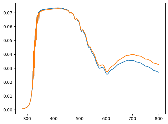
Now we can add in aerosol, let’s set the extinction to be a constant 1e-7 per metre until 30 km, and then zero above that. When we specify our Mie scatterer, we have to make sure to also specify any arguments of the particle size distribution (median_radius and mode_width) as a function of altitudes_m.

aero_ext = np.zeros(len(altitudes_m))
aero_ext[0:30] = 1e-7

atmosphere['aerosol'] = sk.constituent.ExtinctionScatterer(
    mie_db,
    altitudes_m=altitudes_m,
    extinction_per_m=aero_ext,
    extinction_wavelength_nm=745,
    median_radius=np.ones_like(aero_ext)*120,
    mode_width=np.ones_like(aero_ext)*1.6
)

radiance_with_aerosol = engine.calculate_radiance(atmosphere)

And we can plot the results

plt.plot(
    wavel, radiance_no_aerosol['radiance'].isel(los=0, stokes=0),
    wavel, radiance_with_aerosol['radiance'].isel(los=0, stokes=0)
)

[<matplotlib.lines.Line2D at 0x785b540e87a0>,
 <matplotlib.lines.Line2D at 0x785b540e8a10>]

If we look at the dataset with aerosol included,

radiance_with_aerosol

<xarray.Dataset> Size: 7MB
Dimensions:                   (wavelength: 520, los: 4, stokes: 1,
                               aerosol_altitude: 66, altitude: 66,
                               ozone_altitude: 50)
Coordinates:
  * wavelength                (wavelength) float64 4kB 280.0 281.0 ... 799.0
  * stokes                    (stokes) <U1 4B 'I'
Dimensions without coordinates: los, aerosol_altitude, altitude, ozone_altitude
Data variables:
    radiance                  (wavelength, los, stokes) float64 17kB 0.000584...
    wf_aerosol_extinction     (aerosol_altitude, wavelength, los, stokes) float64 1MB ...
    wf_temperature_k          (altitude, wavelength, los, stokes) float64 1MB ...
    wf_aerosol_mode_width     (aerosol_altitude, wavelength, los, stokes) float64 1MB ...
    wf_pressure_pa            (altitude, wavelength, los, stokes) float64 1MB ...
    wf_aerosol_median_radius  (aerosol_altitude, wavelength, los, stokes) float64 1MB ...
    wf_specific_humidity      (altitude, wavelength, los, stokes) float64 1MB ...
    wf_ozone_vmr              (ozone_altitude, wavelength, los, stokes) float64 832kB ...

xarray.Dataset

• Dimensions:
  • wavelength: 520
  • los: 4
  • stokes: 1
  • aerosol_altitude: 66
  • altitude: 66
  • ozone_altitude: 50
• Coordinates: (2)
  • wavelength
    (wavelength)
    float64
    280.0 281.0 282.0 ... 798.0 799.0

    array([280., 281., 282., ..., 797., 798., 799.], shape=(520,))

  • stokes
    (stokes)
    <U1
    'I'

    array(['I'], dtype='<U1')

• Data variables: (8)
  • radiance
    (wavelength, los, stokes)
    float64
    0.000584 0.0006189 ... 0.0003521

    array([[[0.00058404],
            [0.00061886],
            [0.00066529],
            [0.00073403]],
    
           [[0.00061342],
            [0.00065041],
            [0.00069992],
            [0.00077372]],
    
           [[0.00065289],
            [0.00069276],
            [0.00074638],
            [0.00082698]],
    
           ...,
    
           [[0.03272288],
            [0.01215714],
            [0.00153388],
            [0.00035563]],
    
           [[0.03263078],
            [0.01212346],
            [0.00152649],
            [0.00035385]],
    
           [[0.03253921],
            [0.01209004],
            [0.00151915],
            [0.00035208]]], shape=(520, 4, 1))

  • wf_aerosol_extinction
    (aerosol_altitude, wavelength, los, stokes)
    float64
    0.0 0.0 0.0 ... 824.9 1.001e+03

    array([[[[   0.        ],
             [   0.        ],
             [   0.        ],
             [   0.        ]],
    
            [[   0.        ],
             [   0.        ],
             [   0.        ],
             [   0.        ]],
    
            [[   0.        ],
             [   0.        ],
             [   0.        ],
             [   0.        ]],
    
            ...,
    
            [[   0.        ],
             [   0.        ],
             [   0.        ],
    ...
             [ 670.00026814],
             [ 759.34574616],
             [ 898.22118845]],
    
            ...,
    
            [[ 392.75934698],
             [ 623.62716135],
             [ 827.30017576],
             [1003.94600935]],
    
            [[ 393.14641454],
             [ 623.19355614],
             [ 826.09613535],
             [1002.26942816]],
    
            [[ 393.53003387],
             [ 622.762678  ],
             [ 824.89535229],
             [1000.59538449]]]], shape=(66, 520, 4, 1))

  • wf_temperature_k
    (altitude, wavelength, los, stokes)
    float64
    0.0 0.0 ... -1.039e-09 -1.264e-09

    array([[[[ 0.00000000e+00],
             [ 0.00000000e+00],
             [ 0.00000000e+00],
             [ 0.00000000e+00]],
    
            [[ 0.00000000e+00],
             [ 0.00000000e+00],
             [ 0.00000000e+00],
             [ 0.00000000e+00]],
    
            [[ 0.00000000e+00],
             [ 0.00000000e+00],
             [ 0.00000000e+00],
             [ 0.00000000e+00]],
    
            ...,
    
            [[ 0.00000000e+00],
             [ 0.00000000e+00],
             [ 0.00000000e+00],
    ...
             [-2.44359237e-08],
             [-2.70893730e-08],
             [-3.09087014e-08]],
    
            ...,
    
            [[-4.29971195e-10],
             [-7.65317362e-10],
             [-1.04868336e-09],
             [-1.27633763e-09]],
    
            [[-4.29527822e-10],
             [-7.62420684e-10],
             [-1.04370403e-09],
             [-1.26997564e-09]],
    
            [[-4.29088709e-10],
             [-7.59546580e-10],
             [-1.03875810e-09],
             [-1.26365423e-09]]]], shape=(66, 520, 4, 1))

  • wf_aerosol_mode_width
    (aerosol_altitude, wavelength, los, stokes)
    float64
    0.0 0.0 0.0 0.0 ... 0.0 0.0 0.0 0.0

    array([[[[0.],
             [0.],
             [0.],
             [0.]],
    
            [[0.],
             [0.],
             [0.],
             [0.]],
    
            [[0.],
             [0.],
             [0.],
             [0.]],
    
            ...,
    
            [[0.],
             [0.],
             [0.],
    ...
             [0.],
             [0.],
             [0.]],
    
            ...,
    
            [[0.],
             [0.],
             [0.],
             [0.]],
    
            [[0.],
             [0.],
             [0.],
             [0.]],
    
            [[0.],
             [0.],
             [0.],
             [0.]]]], shape=(66, 520, 4, 1))

  • wf_pressure_pa
    (altitude, wavelength, los, stokes)
    float64
    0.0 0.0 0.0 ... 2.268e-08 2.759e-08

    array([[[[0.00000000e+00],
             [0.00000000e+00],
             [0.00000000e+00],
             [0.00000000e+00]],
    
            [[0.00000000e+00],
             [0.00000000e+00],
             [0.00000000e+00],
             [0.00000000e+00]],
    
            [[0.00000000e+00],
             [0.00000000e+00],
             [0.00000000e+00],
             [0.00000000e+00]],
    
            ...,
    
            [[0.00000000e+00],
             [0.00000000e+00],
             [0.00000000e+00],
    ...
             [5.16763263e-07],
             [5.71476457e-07],
             [6.49362119e-07]],
    
            ...,
    
            [[9.38720412e-09],
             [1.67085386e-08],
             [2.28950331e-08],
             [2.78652199e-08]],
    
            [[9.37752431e-09],
             [1.66452978e-08],
             [2.27863235e-08],
             [2.77263237e-08]],
    
            [[9.36793753e-09],
             [1.65825499e-08],
             [2.26783431e-08],
             [2.75883136e-08]]]], shape=(66, 520, 4, 1))

  • wf_aerosol_median_radius
    (aerosol_altitude, wavelength, los, stokes)
    float64
    0.0 0.0 0.0 0.0 ... 0.0 0.0 0.0 0.0

    array([[[[0.],
             [0.],
             [0.],
             [0.]],
    
            [[0.],
             [0.],
             [0.],
             [0.]],
    
            [[0.],
             [0.],
             [0.],
             [0.]],
    
            ...,
    
            [[0.],
             [0.],
             [0.],
    ...
             [0.],
             [0.],
             [0.]],
    
            ...,
    
            [[0.],
             [0.],
             [0.],
             [0.]],
    
            [[0.],
             [0.],
             [0.],
             [0.]],
    
            [[0.],
             [0.],
             [0.],
             [0.]]]], shape=(66, 520, 4, 1))

  • wf_specific_humidity
    (altitude, wavelength, los, stokes)
    float64
    0.0 0.0 0.0 ... 3.177e-10 8.528e-11

    array([[[[0.00000000e+00],
             [0.00000000e+00],
             [0.00000000e+00],
             [0.00000000e+00]],
    
            [[0.00000000e+00],
             [0.00000000e+00],
             [0.00000000e+00],
             [0.00000000e+00]],
    
            [[0.00000000e+00],
             [0.00000000e+00],
             [0.00000000e+00],
             [0.00000000e+00]],
    
            ...,
    
            [[0.00000000e+00],
             [0.00000000e+00],
             [0.00000000e+00],
    ...
             [2.58967318e-06],
             [3.08781575e-06],
             [3.93915565e-06]],
    
            ...,
    
            [[5.84051561e-09],
             [2.35845812e-09],
             [3.31185950e-10],
             [8.89353182e-11]],
    
            [[5.73343233e-09],
             [2.31532564e-09],
             [3.24461650e-10],
             [8.71136595e-11]],
    
            [[5.62526977e-09],
             [2.27176359e-09],
             [3.17702327e-10],
             [8.52830538e-11]]]], shape=(66, 520, 4, 1))

  • wf_ozone_vmr
    (ozone_altitude, wavelength, los, stokes)
    float64
    0.0 0.0 0.0 0.0 ... 0.0 0.0 0.0 0.0

    array([[[[0.],
             [0.],
             [0.],
             [0.]],
    
            [[0.],
             [0.],
             [0.],
             [0.]],
    
            [[0.],
             [0.],
             [0.],
             [0.]],
    
            ...,
    
            [[0.],
             [0.],
             [0.],
    ...
             [0.],
             [0.],
             [0.]],
    
            ...,
    
            [[0.],
             [0.],
             [0.],
             [0.]],
    
            [[0.],
             [0.],
             [0.],
             [0.]],
    
            [[0.],
             [0.],
             [0.],
             [0.]]]], shape=(50, 520, 4, 1))

We can see that the model has also calculated the derivatives with respect to the particle size parameters, median_radius and mode_width.

Freezing Distribution Parameters

The above method of creating Mie scattering databases is useful if you want to run calculations over a wide range of the particle size distribution parameters (median_radius and mode_width) in our example. But there are many applications where some or all of these values are fixed and known. In this case we can “freeze” the parameters of the distribution,

distribution = sk.mie.distribution.LogNormalDistribution().freeze(median_radius=160, mode_width=1.6)

Now when we look at the args property of the distribution,

distribution.args()

[]

We see that it is empty, the distribution is not a function of any parameters because they are all frozen.

We can construct the Mie scattering database and inspect it,

mie_db = sk.database.MieDatabase(
    distribution,
    refrac,
    wavelengths_nm=np.arange(270, 1000, 50.0),
)

mie_db.load_ds()

<xarray.Dataset> Size: 109kB
Dimensions:        (wavelength_nm: 15, cos_angle: 128, legendre: 64)
Coordinates:
  * wavelength_nm  (wavelength_nm) float64 120B 270.0 320.0 ... 920.0 970.0
  * cos_angle      (cos_angle) float64 1kB -0.9993 -0.9964 ... 0.9999 1.0
    distribution   int64 8B ...
Dimensions without coordinates: legendre
Data variables: (12/13)
    xs_scattering  (wavelength_nm) float64 120B ...
    xs_total       (wavelength_nm) float64 120B ...
    xs_absorption  (wavelength_nm) float64 120B ...
    p11            (wavelength_nm, cos_angle) float64 15kB ...
    p12            (wavelength_nm, cos_angle) float64 15kB ...
    p33            (wavelength_nm, cos_angle) float64 15kB ...
    ...             ...
    lm_a1          (wavelength_nm, legendre) float64 8kB ...
    lm_a2          (wavelength_nm, legendre) float64 8kB ...
    lm_a3          (wavelength_nm, legendre) float64 8kB ...
    lm_a4          (wavelength_nm, legendre) float64 8kB ...
    lm_b1          (wavelength_nm, legendre) float64 8kB ...
    lm_b2          (wavelength_nm, legendre) float64 8kB ...

xarray.Dataset

• Dimensions:
  • wavelength_nm: 15
  • cos_angle: 128
  • legendre: 64
• Coordinates: (3)
  • wavelength_nm
    (wavelength_nm)
    float64
    270.0 320.0 370.0 ... 920.0 970.0

    array([270., 320., 370., 420., 470., 520., 570., 620., 670., 720., 770., 820.,
           870., 920., 970.])

  • cos_angle
    (cos_angle)
    float64
    -0.9993 -0.9964 ... 0.9999 1.0

    array([-0.999322, -0.996431, -0.991237, -0.983751, -0.973991, -0.96198 ,
           -0.947746, -0.931323, -0.912751, -0.892072, -0.869337, -0.844599,
           -0.817917, -0.789353, -0.758977, -0.726859, -0.693077, -0.657709,
           -0.620841, -0.582559, -0.542955, -0.502121, -0.460156, -0.417159,
           -0.373231, -0.328477, -0.283003, -0.236916, -0.190327, -0.143346,
           -0.096083, -0.048652, -0.001165,  0.046267,  0.093529,  0.140511,
            0.1871  ,  0.233186,  0.27866 ,  0.323414,  0.367342,  0.410339,
            0.452305,  0.493138,  0.532742,  0.571024,  0.607893,  0.64326 ,
            0.677042,  0.70916 ,  0.739537,  0.7681  ,  0.794782,  0.81952 ,
            0.842256,  0.862934,  0.881507,  0.89793 ,  0.912163,  0.924175,
            0.933935,  0.941421,  0.946615,  0.949506,  0.950201,  0.950275,
            0.950407,  0.950598,  0.950848,  0.951155,  0.951518,  0.951938,
            0.952412,  0.95294 ,  0.953521,  0.954153,  0.954835,  0.955564,
            0.95634 ,  0.957161,  0.958024,  0.958927,  0.959869,  0.960847,
            0.961858,  0.962901,  0.963973,  0.965072,  0.966194,  0.967337,
            0.968499,  0.969676,  0.970866,  0.972066,  0.973274,  0.974485,
            0.975698,  0.97691 ,  0.978117,  0.979317,  0.980507,  0.981685,
            0.982846,  0.983989,  0.985112,  0.98621 ,  0.987282,  0.988325,
            0.989337,  0.990315,  0.991256,  0.99216 ,  0.993023,  0.993843,
            0.994619,  0.995349,  0.99603 ,  0.996662,  0.997243,  0.997771,
            0.998246,  0.998665,  0.999029,  0.999336,  0.999585,  0.999776,
            0.999909,  0.999983])

  • distribution
    ()
    int64
    ...

    [1 values with dtype=int64]

• Data variables: (13)
  • xs_scattering
    (wavelength_nm)
    float64
    ...

    [15 values with dtype=float64]

  • xs_total
    (wavelength_nm)
    float64
    ...

    [15 values with dtype=float64]

  • xs_absorption
    (wavelength_nm)
    float64
    ...

    [15 values with dtype=float64]

  • p11
    (wavelength_nm, cos_angle)
    float64
    ...

    [1920 values with dtype=float64]

  • p12
    (wavelength_nm, cos_angle)
    float64
    ...

    [1920 values with dtype=float64]

  • p33
    (wavelength_nm, cos_angle)
    float64
    ...

    [1920 values with dtype=float64]

  • p34
    (wavelength_nm, cos_angle)
    float64
    ...

    [1920 values with dtype=float64]

  • lm_a1
    (wavelength_nm, legendre)
    float64
    ...

    [960 values with dtype=float64]

  • lm_a2
    (wavelength_nm, legendre)
    float64
    ...

    [960 values with dtype=float64]

  • lm_a3
    (wavelength_nm, legendre)
    float64
    ...

    [960 values with dtype=float64]

  • lm_a4
    (wavelength_nm, legendre)
    float64
    ...

    [960 values with dtype=float64]

  • lm_b1
    (wavelength_nm, legendre)
    float64
    ...

    [960 values with dtype=float64]

  • lm_b2
    (wavelength_nm, legendre)
    float64
    ...

    [960 values with dtype=float64]

We can see that the Mie properties are no longer a function of the particle size distribution parameters since they are assumed to be known. In addition when constructing the database we did not have to specify them.

Similarly, to add aerosol in to our SASKTRAN2 atmosphere we no longer have to specify the frozen particle size parameters,

atmosphere['aerosol'] = sk.constituent.ExtinctionScatterer(
    mie_db,
    altitudes_m=altitudes_m,
    extinction_per_m=aero_ext,
    extinction_wavelength_nm=745,
)

In this example we froze all of the distribution parameters, but we could have frozen only one of them

sk.mie.distribution.LogNormalDistribution().freeze(mode_width=1.6).args()

['median_radius']

Using this distribution we would have to specify median_radius when constructing the database and when adding scatterers to the atmsophere.