Weighting Functions

One of the key features of SASKTRAN2 is that it supports algorithmic calculation of weighting functions, i.e. derivatives of the output parameters with respect to input parameters. In essence, we are calculating

\[ w(x) = \frac{\partial I}{\partial x}\]

where \(x\) is an input parameter to the model, such as ozone VMR at the 10 km level, or the Lambertian surface reflectance at 350 nm.

How to Calculate Weighting Functions

For the most part, weighting functions are calculated automatically, completely opaquely to the user. For example, if we set up a simple calculation,

import sasktran2 as sk
import numpy as np

config = sk.Config()

model_geometry = sk.Geometry1D(cos_sza=0.6,
                                solar_azimuth=0,
                                earth_radius_m=6372000,
                                altitude_grid_m=np.arange(0, 65001, 1000),
                                interpolation_method=sk.InterpolationMethod.LinearInterpolation,
                                geometry_type=sk.GeometryType.Spherical)

viewing_geo = sk.ViewingGeometry()

for alt in [10000, 20000, 30000, 40000]:
    ray = sk.TangentAltitudeSolar(tangent_altitude_m=alt,
                                    relative_azimuth=0,
                                    observer_altitude_m=200000,
                                    cos_sza=0.6)
    viewing_geo.add_ray(ray)

wavel = np.arange(280.0, 800.0, 0.1)

atmosphere = sk.Atmosphere(model_geometry, config, wavelengths_nm=wavel)

sk.climatology.us76.add_us76_standard_atmosphere(atmosphere)

atmosphere['rayleigh'] = sk.constituent.Rayleigh()

atmosphere['ozone'] = sk.climatology.mipas.constituent("O3", sk.optical.O3DBM())

atmosphere['no2'] = sk.climatology.mipas.constituent("NO2", sk.optical.NO2Vandaele())

engine = sk.Engine(config, model_geometry, viewing_geo)

and then inspect the output

radiance = engine.calculate_radiance(atmosphere)
print(radiance)

<xarray.Dataset> Size: 50MB
Dimensions:               (wavelength: 5200, los: 4, stokes: 1, altitude: 66,
                           no2_altitude: 50, ozone_altitude: 50)
Coordinates:
  * wavelength            (wavelength) float64 42kB 280.0 280.1 ... 799.8 799.9
  * stokes                (stokes) <U1 4B 'I'
Dimensions without coordinates: los, altitude, no2_altitude, ozone_altitude
Data variables:
    radiance              (wavelength, los, stokes) float64 166kB 0.0007142 ....
    wf_temperature_k      (altitude, wavelength, los, stokes) float64 11MB 0....
    wf_specific_humidity  (altitude, wavelength, los, stokes) float64 11MB 0....
    wf_pressure_pa        (altitude, wavelength, los, stokes) float64 11MB 0....
    wf_no2_vmr            (no2_altitude, wavelength, los, stokes) float64 8MB ...
    wf_ozone_vmr          (ozone_altitude, wavelength, los, stokes) float64 8MB ...

We see several variables in the output: [wf_pressure_pa, wf_temperature_k, wf_ozone_vmr, wf_no2_vmr]. These are the derivatives of the radiance field with respect to the input variables. All of these variables have the same dimensions as the radiance, plus an additional dimension. The additional dimension is the input dimension, e.g. we specified ozone VMR on an altitude grid thus the input dimension is this altitude grid.

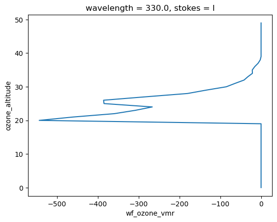
We can take a look at one of the weighting functions,

radiance["wf_ozone_vmr"].isel(los=1, stokes=0).sel(wavelength=330, method="nearest").plot(y="ozone_altitude")

[<matplotlib.lines.Line2D at 0x7c21573784a0>]

The Details

Weighting functions in SASKTRAN2 are calculated analytically, evaluating the derivative of the radiative transfer equation alongside the radiative transfer equation itself in code. This is similar to the “forward mode” of auto-differentiation schemes, however all derivatives in SASKTRAN2 are hand-crafted rather than automatically generated for maximum computational efficiency. Generally you can expect a calculation including full derivatives to be somewhere in the range of 2-5x slower than the calculation without derivatives.

The accuracy of the weighting functions depends on which source terms are included in the calculation. With the exception of the sk.MultipleScatterSource.SuccessiveOrders source, all other sources are “perfectly linearized”, which means that the weighting function calculation is accurate to relative machine precision. Typically we estimate this to be around 6 decimal places for most applications.